Fixed fractional position sizing

The idea behind fixed fractional position sizing is that you base the number of contracts or shares on the risk of the trade. Fixed fractional position sizing is also known as fixed risk position sizing because it risks the same percentage or fraction of account equity on each trade. For example, you might risk 2% of your account equity on each trade (the “2% rule”). Fixed fractional position sizing has been written about extensively by Ralph Vince. See, for example, his book “Portfolio Management Formulas,” John Wiley & Sons, New York, 1990.

The risk of a trade is defined as the dollar amount that the trade would lose per contract if it were a loss. Commonly, the trade risk is taken as the size of the money management stop applied, if any, to each trade. If your system doesn’t use protective (money management) stops, the risk can be taken as the largest historical loss. This was the approach Vince adopted in his book Portfolio Management Formulas.

The equation for the number of contracts in fixed fractional position sizing is as follows:

N = f * Equity / |Trade Risk|

where N is the number of contracts, f is the fixed fraction (a number between 0 and 1), Equity is the current value of account equity (i.e., the value of account equity just prior to the trade for which you’re calculating N ),Trade Risk is the risk of the trade for which the number of contracts is being computed. The vertical bars ( | ) mean that we take the absolute value of the trade risk (risk is usually given as a negative number, so we make it positive).

As an example, consider the series of trades below. The starting account size was $50,000. The profit/loss per contract is shown in the second column (“PL/Contr”). The next column is the trade risk — $320.28 in this case. The fixed fraction was 0.05 (5%). The next column shows the number of contracts computed according the equation above. Multiplying the number of contracts by the profit/loss per contract results in the position profit/loss (“Pos PL”), which adds to the current equity value to give the new value of account equity, shown in the last column.

 

 

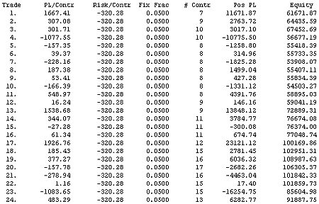
Trades and number of contracts in an example of fixed fractional position sizing.

Notice how the number of contracts tends to increase over time as the profits accumulate. This can also be seen in the figure below, which shows the equity curve and the number of contracts over a longer span of trades from the same market system. The bar chart, below the equity curve, illustrates how the number of contracts drops after a loss and increases after a winning trade.

 

 

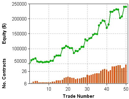
Equity curve and number of contracts in an example of fixed fractional position sizing.

Fixed risk position sizing can be used to implement another one of Vince’s methods, called optimal f position sizing. This is a generalized version of a classic formula called Kelly’s formula , which provides the fixed fraction that maximizes the geometric growth rate for a series of trades where all the losses are one size and all the wins are another size. In this case, the optimal fixed fraction is given by the following equation (Kelly’s formula, as provided by Vince, Portfolio Management Formulas, John Wiley & Sons, New York, 1990):

f = ((B + 1) * P – 1)/B

where B is the ratio of a winning trade to a losing trade, and P is the percentage of winning trades.

O ptimal f position sizing extends the Kelly formula so that the wins and losses can all be different sizes. Optimal f calculates the fixed fraction that maximizes the rate of return for a given series of trades. While this sounds like a good idea, in practice the optimal f value (or the f value from the Kelly formula) often results in drawdowns that are too large for most people to tolerate.

Also, relying on the historical sequence of trades is risky in that the sequence of profits and losses in the future may be less favorable than what was encountered historically. As a result, the drawdowns in the future could be much larger than predicted by the historical sequence of trades. Performing a Monte Carlo analysis on the trade sequence is one way to generate a more conservative estimate of the future worst-case drawdown.

A less risky alternative to optimal f is to optimize using Monte Carlo analysis and with a specified limit on the maximum allowable drawdown. This will generally yield a much smaller and therefore less risky fixed fraction than optimal f.

 

Reprinted with permission Michael Bryant (www.adaptrade.com)