Ito Calculus

This tutorial written and reproduced with permission from Peter Ponzo

 

Kiyosi Ito studied mathematics in the Faculty of Science of the Imperial University of Tokyo, graduating in 1938. In the 1940s he wrote several papers on Stochastic Processes and, in particular, developed what is now called Ito Calculus.

I haven’t the faintest idea …

Patience. I’m getting to that. Do you remember when we talked about Random Walks?

Uh … no.

Well, we got a formula for the change in (for example) a stock price after n days (or weeks or months):

[1]  P(n+1) – P(n) = r P(n) 

where r is the daily (or weekly or monthly) gain.

And r is a constant?

We could, of course, assume that it’s a constant in which case:

P(n+1) = (1+r)P(n) so that:

      P(1)=(1+r)P(0) 
      P(2)=(1+r)²P(0) 
      P(3)=(1+r)³P(0) 

and, at time “n” 

      P(n)=(1+r)ⁿP(0)

as in Figure 1.

 

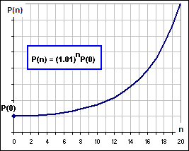
Figure 1

I’ll take it!

On the other hand, we could assume that r changes, day to day.

Or week to week or month to …

Yes, yes. Let’s just say from one time to the next. That’d change our equation [1] to:

[2] P(n+1) – P(n) = r(n) P(n)

Now we’d expect r(n) to be random … but not entirely.

Huh?

Do you remember when we talked about

Uh … no.

Well, we suggested that the gains, from one time period to the next, have a deterministic component and a random component. Let’s do that here, writing:

[3] P(n+1) – P(n) = [d(n) + s(n)] P(n)

where d(n) is the deterministic part and s(n) is the random part. For example, in Figure 2, the upper and lower charts show a deterministic and a random component. Add them together and you get

 

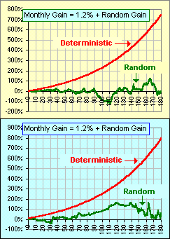
Figure 2

 

 

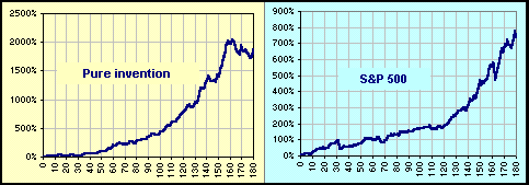
See? Although one is pure invention, the other is fifteen years of the S&P 500.

In [3], why do you say s(n) ? Why not r(n) for random?

We’ve used r(n) already … so s(n) means stochastic component which sounds far sexier, eh? Anyway, we’ll rewrite [3] like so:

P(n+1) – P(n) = d(n) P(n) + s(n) P(n)

and, if we put DP = P(n+1)-P(n) and assume that time progresses continously (so the change in time is not “1”, from n to n+1, but Dt) we get something which looks like:

[4] DP = m(t,P)Dt + RDt

where m(t,P) is some known/deterministic function which depends upon the time. (which we’re now calling “t” instead of “n”) and the current price “P” and …

And R has all the random stuff, eh?

Yes. All the stochastic stuff.

And you just stick in that Dt, eh? I wasn’t there before, but now it’s there.

Well .. uh, [3] actually gives the Rate of Change over a time length of “1”. See? P(t+1) – P(t) is the change over a time interval of length “1”.  It’s {P(t+1) – P(t)}/Dt with Dt = 1. But, if Dt isn’t “1′, but much smaller, then we’d want to have {P(t+Dt) – P(t)}/Dt … so [3] would become {P(t+Dt) – P(t)}/Dt = [d(t) + s(t)] P(t). Multiply by Dt and we’d get our [4]. See?

 

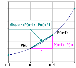
Figure 3

 

Huh? Dt is much smaller? Why?

Remember, we’re now talking NOT about time which advances day by day or week by week, but second by second. A continuous time progression.

Yeah, so where does Ito come in?

Equation [4] is Ito’s stochastic equation.

That’s it?

Hardly. We’ve got to investigate that stochastic term which we’ve called RDt. Let’s rewrite equation [4] like so:

[Ito-1] DP /Dt = m(t,P)+ R

First, note that the random term (which we denote by R) is the stochastic component for DP /Dt (or, for those who get turned on with calculus, this would be dP/dt), the Rate of Change in stock price. Next, we expect this term to have some Mean and Standard Deviation. What are they? We stare at a chart of, say, the S&P 500 over several years. It’s easy enough to split the prices (over time) into two parts so that they add to the exact S&P 500.

Huh?

Look at Figure 2, the lower chart. There’s a smooth red curve and green, random component. Add them together and we get the S&P chart. However, we could just as easily have chosen different smooth and random components which add to the actual S&P 500. How should we identify the …

Will the REAL random component please stand up!

Well … yes, so we look at [Ito-1] and see that we should be looking at the Rate of Change of the price. Okay. Suppose we:

Assume a smooth growth at the rate r (where r = 0.123 means 12.3%).
That would give P(t) = P(0)(1+r)t.
That would make the Rate of Change dP/dt = log(1+r) P(t), hence is proportional to P(t).
Now compare this “smooth” Rate of Change with the actual Rate of Change.
That is, generate the Difference in dP/dt, from one time to the next.

For a couple of values of r, we get the following pictures (using the annual S&P prices over the interval 1928 – 2000):

 

 

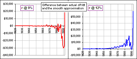
So that suggests that we choose r so that …

The difference is zero!

Well, not zero, but with an Average, or Mean, of zero. We can play with the r-values and get r = 0.1072 corresponding to 10.72% … as shown in Figure 4.

 

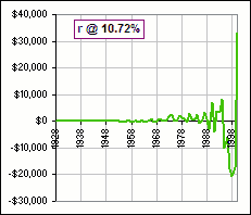
Figure 4

How does that 10.72% compare with the …

It actually turns out to be the annualized return over the period 1928 to 2000.

Is that always the case?

No. We’re not considering the deviation of Prices but the deviation of Rates of Change of Prices. For example, let’s consider the same fifteen year period as we did in Figure 2. We suppose we start with $100 and invest in the S&P 500 and look at the value of r which makes the average Difference in dP/dt equal to zero. It turns out to be r = 0.0020 or 0.20% per month. On the other hand, the compound monthly return (over the fifteen year period) is 0.21% per month.

So why don’t you make the average error equal to $0

… between the actual price and that smooth price? This isn’t MY methodology. It’s Ito’s. What do I know? I just try to explain what others have done. I don’t do my own stuff, I just regurgitate and …

 

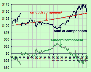
Figure 5

Picture?

Okay, the smooth and random components are shown in Figure 5, using that monthly return of 0.20%.

What if you use that 0.21%? The one that makes the average error equal to $0.

The error between the actual price and that smoothed price? It’s in Figure 5. Look closely. It’s the faint grey curve. Can you see it?

No.

Don’t worry about it. In any case, we’re going to choose that random component so that it has a Mean of zero. That is, the Expected value of R is zero. That is E[R] = 0.

We are going to choose? Who’s doing the choosing?

Uh … Kiyosi Ito. Okay, let’s continue. Although there are several forms for Ito’s equation, which we’ve written as DP /Dt = m(t,P)+ R, we’ve chosen to write the Random term as, simply, R so as to embrace all forms (I hope). Further, since we’re talking about continuous time progression, we’ll set DP /Dt = dP/dt.

Now we’ll rewrite Ito’s equation like so:

[Ito-2] dP = m(t,P)dt+ s(t,P) df(t)

where f(t), which gives rise to the term df(t), is a Brownian Motion.

Huh?

f(t) goes up or down at random. The next incremental step is independent of the previous step. The motion has no memory. The path is a continuous random walk. It provides the stochastic component for our Price changes.

Please continue.

Okay, as a simple example, suppose we set m(t,P) = aP and s(t,P) = 1 and df is a random variable with Mean = 0 and Standard Deviation = 1.

What if df = 0? Isn’t that even simpler?

Yes, then we’d have dP/dt = a P which is an ordinary differential equation with solution: P(t) = P(0)eat and the graph of this function is the same as shown in Figure 1. In fact, if a = log(1+r), then P(0)eat = P(0)(1+r)t … which we’ve seen before.

That’s the smooth part. If we include that df term we’d get …

Yes, exactly. We’d get an additional, random component.

So do it!

Well … that’s not so easy. One rarely solves equations like [Ito-2], however there are some interesting things we can do …

Will you talk about f(t), that Brownian stuff?

Patience.