Black Litterman
This tutorial written and reproduced with permission from Peter Ponzo
Once upon a time, in 1952, Harry Markowitz introduced “Modern Portfolio Theory” and the “Mean-Variance optimization” and …
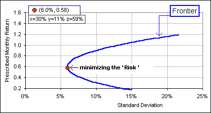
Figure 1
Huh?
You pick a “risk” which you’re comfortable with (they equate Risk = Standard Deviation), then vary your asset allocation (hence your expected return) so your portfolio is represented by a point on a so-called Efficient Frontier. Or maybe you want to minimize Risk so …
Huh?
I don’t want to talk about Frontiers. I want to talk about a more recent prescription for calculating some kind of optimal allocation: the Black-Litterman Model.
What’s wrong with Frontiers?
Don’t ask me! How would I know? I just read about this stuff and write …
Yeah, yeah … so what’s wrong with Frontiers?
Apparently, the suggested “Frontier” allocation is sometimes unexpected, non intuitive, ignores current market conditions, is very sensitive to small changes in …
What does that mean?
See Figure 1? That’s a real, live example where there are three assets: the S&P500, U.S. Small Cap and Gold. We vary the percentage allocated to these three assets so as to minimize our “Risk”.
Where Risk = Standard Deviation, right?
Right. You get (as indicated in Figure 1) 30% S&P, 11% Small Cap and 59% Gold. See the red dot?
What? 59% Gold!?
Currently, gold is very volatile so we wouldn’t expect to place that much …
Can we go on to Black-Litterman now?
Yes, but before we do that, let’s see how sensitive that Frontier technique is when you make small changes in the parameters. Here’s a Mean-Variance optimization spreadsheet with three assets. Each has some mean annual return … and a there’s a bunch of correlations/covariances.There’s also a “required” annual portfolio return.
We want to use the Efficent Frontier to determine the asset mix that’ll minimize the Variance = (Standard Deviation)2 of our portfolio, while providing the “required” annual return.
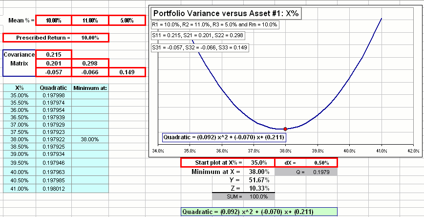
So I make small changes in the numbers and I’m supposed to notice an unexpectedly large change in allocation, right?
Yes. Try changing the annual return for Asset #1, from 10% to 11%.
Can we go on to Black-Litterman now?
With Black-Litterman (developed while Fischer Black and Robert Litterman were at Goldman Sachs, in the 1990s) we have an opportunity to insert expected performance, based upon observation of current market conditions and our view of the market … maybe bullish, maybe bearish.
And if I don’t have any views on the market?
If you have absolutely no views (like A will outperform B by 2%), then you hold the market itself … like maybe an Index Fund.
Is that what Black-Litterman says?
I think so, but I’m still learning … and staring intently at a Black-Litterman formula I found on the Net:
![]()
Mamma mia!
Ya took the words right outta my mouth.
An Allocation Model
Our job is to understand that Black-Litterman formula. It supposedly gives the expected returns of the various portfolio assets in terms of their “implied” returns and correlations and our views on the assets as well as our confidence in those views.
Do people actually use it?
Did I mention that it was developed at Goldman-Sachs, one of the world’s oldest and most prestigious investment banks?
Yeah, so what does it mean?
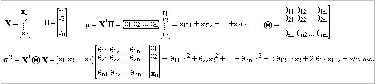
Patience: Our portfolio is allocated among n assets, with expected, future excess returns (above some risk-free rate): r1, r2, … rn. We devote fractions to each asset, namely: x1, x2, … xn (where x1+x2+ …+xn = 1). Our expected portfolio return is then: x1r1 + x2r2 + … +xnrn. Introduce the n x 1 vectors: X = [x1, x2, … xn] and Π = [r1, r2, … rn] so our expected portfolio return is: μ = XT Π.
Huh?
XT is the transpose of the vector X. We’re talking matrix multiplication here. Let the covariance matrix associated with the n assets be: Θ The variance of our portfolio is then: σ2 = XT Θ X = θ11x12 + θ22x22 + … + θnnx12 + 2 θ12 x1x2 + 2 θ13 x1x2 + … etc. etc.
Beg pardon?
Okay, lets’ write this stuff in a more familiar format:
Now, if our portfolio has a mean return μ and variance σ2 , its long term annualized return is (approximately) : μ – (1/2) σ2. What we’ll do is attempt to optimize μ – (λ/2) σ2 by clever choice of the allocation vector, X.
What’s that λ?
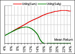
Remember when we talked about utility functions?
No!
Well, read all about it.
In particular, Sam was less concerned than Sally with the volatility of his portfolio, … so he took as his utility function: μ – (0.5/2) σ2. Sally, on the other hand, was more conservative and appalled by large volatility, … so she took as her utility function: μ – (10/2) σ2.
Here, we won’t commit ourselves but just assume some risk-aversion parameter λ and take as our utility function:
U(X) = μ – (λ/2) σ2 = XT Π – (λ/2) XT Θ X = Σ xk rk – (λ/2) Σ xi θij xj
Then, to maximize, we set all partial derivatives to 0:
∂U/∂ xk = rk – (λ/2) Σ 2 θik xk
Hence:
Σ θik xk = rk … for k = 1, 2, … n
In other words:
λ Θ X = Π
Finally, solving for our allocation vector:
X = (1/λ) Θ-1 Π
Our expected return is then:
μ = XT Π = (1/λ)Π’Θ-1 Π
Let’s give this a place distinction:
Magic Formula:
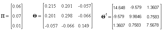
If Π is the n-vector of portfolio returns, and
X is the n-vector of asset allocations, and
Θ is the n x n (symmetric) covariance matrix
then the optimal allocation of assets is X = (1/λ) Θ-1 Π
and the resultant, expected return is given by: μ = XT Π = (1/λ)Π’Θ-1 Π
where λ is a user-selected risk-aversion scalar.
zzzZZZ
Don’t fret. We’ll (eventually) have a spreadsheet to do the dirty work. In the meantime, note that Π, what we’re calling “returns”, is really expected excess asset returns.
Note, too, our ritual might do this:
Assume some utility function U which depends upon the asset weights X and a set of parameters (characterized above by Π and Θ).
Let the set of parameters be denoted by ζ. Then we write U(X|ζ), meaning the dependence of U on the asset weights X, given the set of parameters ζ.
We vary X so as to maximize E[U(X|ζ)], the Expected value of U, given the parameters ζ.
We could assume the parameters are known, say from historical data. Alas, the future ain’t usually like the past.
We then regard historical data (for example) as a sample which provides an estimate of the true parameter values.
From this sample we attempt to generate an estimate of the true values of the parameters … as opposed to assuming we know them!
If the “sample” parameters are denoted by ζ’ (as opposed to the true parameter values which we’ve denoted by ζ) then we maximize E[U(X|ζ’)]
Since ζ’ is not the true value of the parameters (except by accident!), our maximization will provide a suboptimal allocation of assets.
In order to see how well our “sample” did in generating the optimal allocations, we introduce an Error Function:
1 – max{E[U(X|ζ’)]} / max{E[U(X|ζ)]}
Huh?
If the real utility maximum is 1.23 and the maximum we obtain with our sample parameters is 1.11, them the error is: 1 – 1.11/1.23 = 0.10 or 10%.
But … uh, to calculate the error you gotta know the real maximum!
Yeah. True, but math types have ways to circumvent this. Remember that we really want the true value of those parameters (and we wisely refuse to accept the historical values).
Realizing that we hate uncertainty (or volatility), we could consider the worst-case scenario where the parameters are chosen to minimize the utility function. That is, select ζ so as to minimize: U(X|ζ). Call this minimizing set of parameters ζ’. The, having this worst-case utility, determine the best possible alloaction.
That is, select X so as to maximize: U(X|ζ’)
The neat thing about Black-Litterman is assuming some “equilibrium” market parameters (in which we have great faith) then allow our portfolio parameters to deviate from the market parameters … and assign some confidence level to the deviations.
Confidence level?
Remember when I referred to “… our views on the assets as well as our confidence in those views.” Well, here’s where that fits in.
Yeah, sure. I can hardly wait, but what about that other model where you already have the answer? Is it any good?
You mean X = (1/λ) Θ-1 Π
Okay, let’s try it for three assets. We’ll use the same parameters as we used above, namely:
R1 = 10%, R2 = 11%, R3 = 5% and our risk-free rate will be, say 4%. Then the excess returns are: r1 = 0.06, r2 = 0.07 and r3 = 0.01 (where we change to decimals). Okay, so our return vector and covariance matrix (and its inverse) look like this:
Then gives the allocation ratios.
But shouldn’t they add up to 1?
Oh, yes. I forgot to tell “the Math” that x1 + x2 + x3 = 1. The sum of ratios obtained above is 1.2286 so we divide each ratio by that sum and get:
x1 = 34.0%, x2 = 17.8% and x3 = 48.2% (changing again to percentages).
What happened to λ?
In this allocation model, it cancels out … in the process of normalizing the allocation ratios (so they add to 1). In fact, when we set all the derivatives to 0, it’s saying that there are no constraints on the values of the xk. In particular, they need not add to “1”.
Aren’t we doing Black-Litterman.
Not yet, but …
So why doesn’t it give the same result as we got above, with the same parameters?
That was mean-variance Frontier stuff, where we specified our portfolio return. Besides, the returns weren’t excess returns. We wouldn’t expect …
You said there’d be a spreadsheet!
Yes and here it is where we stick in the same returns as we did above (ignoring the fact that we’re supposed to be using excess returns). That way we can compare to the result we got above:
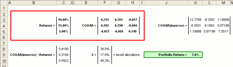
Click on the picture to download the spreadsheet. Fill in the Returns and enter the Covariance matrix and …
Covariance matrix? And where do I find that guy?
You can try the spreadsheet described here. Anyway, the above the spreadsheet does the rest … giving you the allocation vector X. Note that the portfolio return is 7.8%.
So if I do that earlier thing and ask for a 7.8% return, I’d get the same allocations?
Try it. Change the Required Annual Return to 7.8% in the spreadsheet.
So I get the Frontier result, right?
Right.
So where’s Black-Litterman?