Linear Regression

This tutorial written and reproduced with permission from Peter Ponzo

We assume that some set of variables, y₁, y₂, … y_K, is dependent upon variables x_k1, x_k2, … x_kn (for k = 1 to K). We assume the relationship betwen the ys and xs is “almost” linear, like so:

[1]
y₁ = ß₀ + ß₁x₁₁ + ß₂x₁₂ + … +ß_nx_1n + e₁
y₂ = ß₀ + ß₁x₂₁ + ß₂x₂₂ + … +ß_nx_2n + e₂
……..
y_K = ß₀ + ß₁x_K1 + ß₂x_K2 + … +ß_nx_Kn + e_K

Why so many variables?

Well, suppose we note that, when the xs have the values x₁₁, x₁₂, … x_1n, the y-value is y₁. We suspect an almost linear relationship, so we try again, noting that x-values x₂₁, x₂₂, … x_2n result in a y-value of y₂. We continue, for K observations, where, for x-values x_K1, x_K2, … x_Kn the result is a y-value of y_K. Then in an attempt to identify the “almost” linear relationship, we assume the relationship [1].

We can write this in matrix format, like so:

[2]

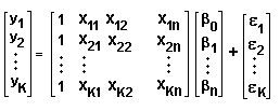
or, more elegantly:

[3]
y = Xß + e 

where y, ß and e are column vectors and X is a K x (n+1) matrix.

We attempt to minimize the sum of the squares of the errors (also called “residuals”) by clever choice of the parameters ß₀, ß₁, … ß_n.

E = e₁² + e₂² + …+e_K² = e^Te     where the row vector e^T denotes the transpose of e.

(Note that this sum of squares is just the square of the magnitude of the vector e … so we’re making the vector as small as possible.) We set all the derivatives to zero, to locate the minimum.

For each j = 0 to n we have:

?E / ?ß_j = 2 e₁ ?e₁/?ß_j + 2 e₂ ?e₂/?ß_j + … + 2 e_K ?e_K/?ß_J = 2 S e_k ?e_k/?ß_j = 0     
the summation being from k = 1 to K.

Since ek = yk – ß0 – ß1xk1 – ß2xk2 – … – ßnxkn   (from [1]) then:

e_k ?e_k/?ß_j = [y_k – ß₀ – ß₁x_k1 – ß₂x_k2 – … – ß_nx_kn] (-x_kj) = -(x_kj)* [y_k – ß₁x_k1 – ß₂x_k2 – … – ß_nx_kn]

= -(the kjth component of X)*[the kth component of y – Xß]
= -(the jkth component of XT)*[the kth component of y – Xß]

then we have n+1 equations (for j = 0 to n) like:

[4]
Sek ?ek/?ßj = – S(the jkth component of XT)*[the kth component of y – Xß]   … summed over k.

But [4] defines the jth component of the n-component column vector: XT [ y – Xß ]. Setting them to zero gives us n+1 such linear equations to solve for the n+1 parameters ß0, ß1, ß2 … ßn, namely:

[5]       XT [ y – Xß ] = 0.

What about the xs and ys?

We know them. They’re our observations and our goal is to determine the “almost” linear relationship between them. That means finding the (n+1) ß-values which we do by solving [5] for:

[6]       ß = (XTX)-1XTy   where (XTX)-1 denotes the inverse of XTX.

Don’t you find that … uh, a little confusing?

It’ll look better if we elevate it’s position like so:

If we wish to find the “best” linear relationship between the values of y₁, y₂, … y_K and x_k1, x_k2, … x_kn (for k = 1 to K) according to:

y₁ = ß₀ + ß₁x₁₁ + ß₂x₁₂ + … +ß_nx_1n + e₁
y₂ = ß₀ + ß₁x₂₁ + ß₂x₂₂ + … +ß_nx_2n + e₂
……..
y_K = ß₀ + ß₁x_K1 + ß₂x_K2 + … +ß_nx_Kn + e_K

or

or

y = Xß + e

where the K-vector e denotes the errors (or residuals) in the linear approximation, y is a K-vector, ß an (n+1)-vector and X a K x (n+1) matrix, then we can minimize the size of the residuals by selecting the ß-values according to: ß = (XTX)-1XTy

Well it doesn’t look better to me!

Here’s an example where K = n = 3 and ß0 = 0 (so we’re looking for ß1, ß2 and ß3 and we ignore that first column of 1s in X):

 

 

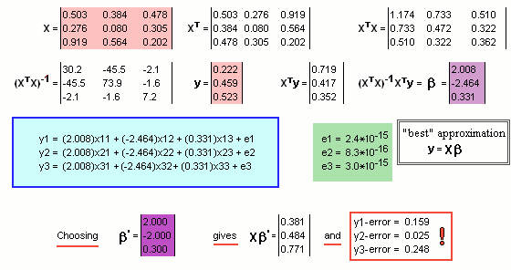
Note the assumed values for the X matrix and the column vector y … coloured 

We run thru’ the ritual, calculating XT and XTX etc. etc. … and finally the ß parameters … coloured 

The resultant (almost linear) relationship is inside the blue box.

There are (as expected!), errors denoted by e1, e2 and e3 … but they’re pretty small. They’re coloured 

If, instead of those “best” choices for the parameters, we had chosen a different set, say ß’   coloured  the errors are significantly greater.