Utility Theory (Part 2)

This tutorial written and reproduced with permission from Peter Ponzo

We’re attaching a personal “Utility” to the prospect of receiving $x, namely U(x). For example, we might choose the Utility Function U(x) = SQRT(x) so that we attach to a gain of $10,000 a “Utility” of SQRT(10,000) = 100 and we attach a utility of SQRT(100) = 10 to a gain of $100 and we attach …

Okay! I get it! So tell us if this is a useful idea … please!

Okay, but note that for the above Utility Function, winning $10,000 is not a hundred times more valuable than winning $100. This square-root utility function makes it only ten times more appealing.

Oh yeah? Well, I find it a hundred times more appealing.

So you’d be willing to pay 100 times more money for the chance to win $10,000 … as opposed to winning $100?

Of course not!

Aah … that’s the point. It’s all about your personal risk profile, about your personal …

If you gave me an example, I might understand this mumbo jumbo.

Okay, consider the following problem:

Sam is willing to take risks in order to achieve (possibly) greater returns, even if there’s a greater chance of losing. Sally is risk averse and would rather achieve a smaller return, with its smaller associated probability of losing money. They each must determine how much of their investment should be devoted to assets A or B.

Asset A has an mean return of M = 20% and a Standard Deviation of S = 34% 
Asset B is a risk-free asset with M = 4% and a Standard Deviation of S = 0% it’s risk-free?

Now we pick Utility Functions for Sam and Sally which reflect their risk tolerance:

Before we proceed, let’s talk a bit about the relation between expected Annualized return A, Mean return M and Standard Deviation S. For a given Mean return, the Annualized return decreases with increasing Standard Deviation. The more volatile the investment, the less the expected Annualized return. In fact, a good approximation for the Annualized return is:

(1)     A = M – S2/2

 

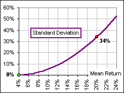
Figure 1

 

Let’s assume, as in Figure 1, that there’s a range of assets with increasing Mean return and, associated with each, a corresponding Standard Deviation which increases rather dramatically. For example, at M = 4%, we have a risk-free return (with S = 0) and, at a Mean of 20%, the Standard Deviation is 34%. The Annualized returns associated with this collection of investments, using equation (1), is shown in Figure 2.

 

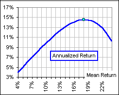
Figure 2

 

Note that, because of the dramatically increasing Standard Deviation, the Annualized return begins to decrease when the Mean return exceeds 18%. Okay, now we’re in a position to generate a Utility Function for Sam and Sally: Sam is less concerned with volatility (that’s S2), so, in place of equation (1), he takes as his Utility Function

(2)     U(Sam) = M – 0.5 S2/2 with less weight for the second term

Sally, on the other hand, is appalled by huge volatilities and weights the second term more heavily, like so:

(3)     U(Sally) = M – 10 S2/2

and attributes a Utility of “0” when the Mean (hence Standard Deviation) is too large. The two Utility Functions are shown in Figure 3.

 

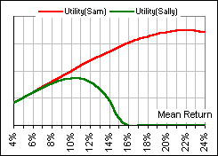
Figure 3

 

I’m with Sam. The bigger the annualized return, the more weight he gives!

Yes, and the greater chance of losing money. Okay, now we ask Sam and Sally to divide their investment monies between two assets, A and B.

Who’s A? And B?

You’ve forgotten already?

Asset A has an mean return of M = 20% and a Standard Deviation of S = 34% 
Asset B is a risk-free asset with M = 4% and a Standard Deviation of S = 0%

If you assign a fraction x to asset A and the balance (1-x) to asset B, then the Mean return of your portfolio is

(4)     M = x (0.20) + (1-x) (0.04)  a combination of the two Mean returns of 0.20 (or 20%) and 0.04 (that’s the 4%) and the Standard Deviation of your portfolio is

(5)     S = x (0.34)  only asset A contributes to the Standard Deviation of 0.34, since asset B has S = 0

Sam then stares at his Utility Function (from (2), above, using M and S from (4) and (5)):

(6)     U(Sam) = {x (0.20) + (1-x) (0.04)} – 0.5{x (0.34)}2/2

… and Sally does likewise, using (3):

(7)     U(Sally) = {x (0.20) + (1-x) (0.04)} – 10{x (0.34)}2/2

Do you have a picture? A picture is worth a thousand …

Yes, here’s a picture (Figure 4) which gives the Utility which each places on an allocation of a fraction x to asset A:

 

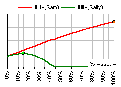
Figure 4

 

Are you saying that Sam allocates 100% to asset A?

Yes, and Sally allocates just 15%.

I think Sam is going a bit overboard. I think …

You’d take a somewhat more conservative Utility?

Me? I’d take U(me) = M – 2 (S2/2)

Instead of M – 0.5 (S2/2)? Okay. You’d devote about 70% to asset A, like it shows in Figure 5

 

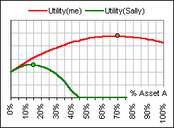
Figure 5

 

I’ll take it!

Actually, if you pick a “Risk Aversion Number”, M, from 1 to 10 (the bigger the number the LESS risk you’d be willing to take) then the percentage stock you’d choose is given by:

Percentage Stock = { Mean(stock) – Mean(risk-free) } / { M SD2(stock) }

We’re talking … what Utility?

We’re talking:

U(x) = x Mean(stock) + (1-x) Mean(risk-free) – M {x SD(stock)}2/2

For example, you may want to play with the calculator shown here.

 

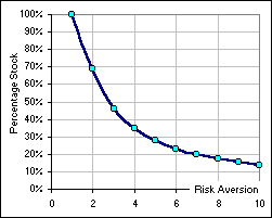
Figure 5a

 

Well, there are lots of possible Utility Functions. For example, in Part I, we noted some characteristics, shown in Figure 6. In particular, look at the Risk Averse utility function (in blue). That’s the one most  investors would appreciate. Indeed, look again at Figures 4 and 5, above. You and Sam were both happy with some risk, but you wanted a lesser risk than he … and that was reflected in your Utility Function: it has a greater downward curvature.

 

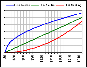
Figure 6

 

Yeah, but look at Sally’s curves!

Careful what you say … Anyway, everybuddy has his/her favourite Utility. Here’s a popular choice:

A Constant Relative Risk Aversion (CRRA) utility

 

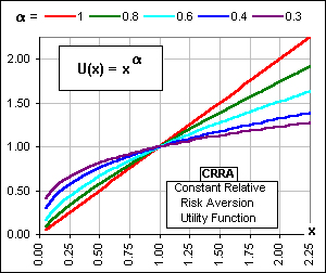
Figure 7

 

Note that choosing a = 1/2 gives the SQRT(x) Utility.

Why is it called Constant Relative Risk Aversion?

You don’t want to know.

Sure I do.

Okay, it assumes a Relative Certainty Equivalence which implies that

x U”(x)/U'(x) = constant and this differential equation has solutions …

You’re right. I don’t want to know.

Okay, here’s a neat example of Utility:

You have a $100 portfolio and start tossing a coin. If it comes up Heads, you increase your holdings by 25%. If it comes up Tails, you lose 10%. What’s the Expected Value of your holdings after ten tosses?

What’s that got to do with Utility?

Patience. Remember the Binomial Distribution?

No. In fact …

Pay attention. For 10 tosses, there are 210 = 1024 possible sequences of Heads and Tails. Every time you get a Head, you multiply by 1.25 and every time you get a Tail you multiply by 0.9. You could get 10 Heads, in which case your $100 nest egg would grow to 100 (1.25)10 = $931.32 or 9 Heads and 1 Tail in which case you’d have 100 (1.25)9(0.9)1 all the way to 10 Tails in which case you’d have 100 (0.9)10 = $34.87

That’s less than a dozen ways to toss the coin. You said 1024 ways.

Yes, but there are 10 ways just to do the 1-Head scenario. That 1 Head could be on the 1st or 2nd or 3rd toss, etc.. For example, there are 120 ways to get 3 Heads and 7 Tails. In fact, the number of ways to get 3 Heads in 10 tosses is 10C3 which is 10!/(3! 7!) = (10 x 9 x 8)/(3 x 2 x 1) = 120

I beg your pardon?

I told you. Read that Binomial Stuff. In any case, since there are 120 3-Head scenarios out of 1024, there’s a probability of 120/1024 = 0.1172 or 11.72% of getting one of these.

 

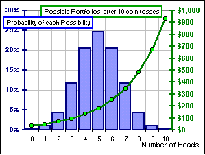
Figure 8

 

In this way we can calculate the Probability of getting any of the 0-Head, 1-Head, etc. sequences and for each such sequence of Heads and Tails there’s a Value for our portfolio, after 10 tosses … as we see from Figure 8. Hence, knowing the Probability and the Value for each we can …

Don’t tell me! It’s that Probability x Value again.

It’s the sum of Probability x Value and the various Probability x Value numbers are shown in Figure 9. It turns out that the SUM is $206.10 and that means …

 

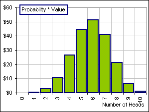
Figure 9

 

It means my $100 grew by a Gain Factor of 2.061

Over 10 tosses. Per toss, it’s 2.061(1/10) or 1.075 and that means an expected return of 7.5% per toss, right?

Where does Utility come in?

So far we’ve assumed that we value $100 twice as highly as $50 and $150 three times as highly as $50 … the Utility we assign to each Value is the Value itself. In other words, U(x) = x. But suppose you’re given a choice between a constant gain of 5% for each coin toss (that means multiply your $dollars by 1.05 every time you toss the coin, giving you 100 (1.05)10 = $162.89 after 10 tosses) or the +25% and -10% scenario we described above. Which do you choose?

I choose the latter because 7.5% is better than 5%. Am I right?

But the 5% is guaranteed whereas the 7.5% is some kind of average gain. You could, with 10 straight Tails, wind up with just $34.87, a loss of about 65%.

Okay, I pick the guaranteed 5%. Am I right?

We’ll see …