Black Scholes

This tutorial written and reproduced with permission from Peter Ponzo

Here, we want to describe the logic behind the Black-Scholes Option Pricing Formula which looks like this:

 

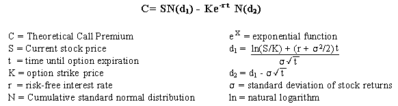
Figure 1

What do all those symbols …?

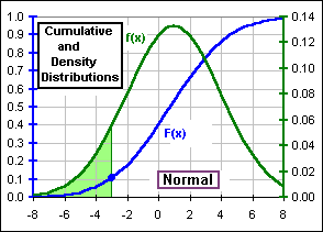
We’re not going to derive the formula … just give some indication of how it arises. We’ll be talking about a cumulative distribution function, F(x), and its derivative, f(x), the density distribution. Typical charts might look like this where the slope of the F-curve, namely dF/dx, is the f-curve and the area beneath the f-curve is the F value.

 

 

If x is a random variable (distributed according to some distribution, as shown), then the Mean or Expected value of x is E[x] = . Further, if we want to know the Mean or Expected value of some Quantity that depends upon x, say Q(x), then it’s E[Q(x)] = . In particular, the squared deviation of the x’s from their mean, namely (x-m)², has an Expected Value of  which we recognize as the square of the Standard Deviation.

We do?

Yes. In fact …

Just what’s the purpose of all this?

Okay, let’s just plunge right in: We know that, at expiry of a Call Option, if S is the stock price and K is the Strike Price then the Option is worth S – K provided S is greater than K … or it’s worth nothing (if S is less than K). In other words, the Option Price (at expiry) is the maximum of S – K or 0, namely:

(1) C = Max(S – K, 0)

Ah, but that’s at expiry of the Option. If the Option expires t years (or months or weeks) in the future, what’s the Option worth now? Suppose that, t years in the future, the stock price is x. Then the Option, at expiry, is worth C_t = Max(x – K, 0), according to Equation (1). The Expected Value of this Quantity, assuming some distribution of yearly (or monthly or weekly) stock returns, is then

(2) E[C_t] = E[Max(x – K, 0)]

which we recognize as  =  where we integrate from K since Max(x – K,0) is zero when x < K.

If that’s the Expected value of the Option at expiry, then what’s the expected value now, today, this very minute?

It’s the Present Value of E[C_t], assuming a risk-free rate of, say, r. That means it’s worth

(3) C = e^-rt E[C_t] or simply e^-rt 

or

(4) C = e^-rt  – K e^-rt  = e^-rt – K e^-rt {1 – F(K)}

where F is the cumulative distribution.

Where did that e^-rt come from?

Well, if we were to put $A in the bank at an interest rate of r, then, after t years, it’d be worth B = A{1+r}^t so A = B {1+r}^-t gives the Present Value of $B.

And where did e^-rt come from?

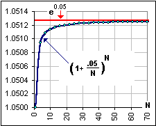
We assume continuous compounding, so if we subdivide a year into N periods, the interest rate for each period is r/N and the number of periods is N so we have (1+r/N)^N as the yearly growth, at the annual rate r … if the compounding is continuous.

And where did e^-rt come from?

(1+r/N)^N approaches the value er, as N approaches infinity – that’s a well known theorem. Anyway, that’s the meaning of continuous compounding. Here’s an example with r = 0.05 (meaning 5%):

 

A well known theorem?

Yes. Now, instead of {1+r} as the annual growth factor, we use {er} and so {1+r}-t becomes {er} ^-t which is e^-rt, so the present Value is written as C_t e^-rt … instead of C_t = C{1+r}^-t.

Sounds like mumbo-jumbo to me.

The math is much, much nicer. Besides, this calculation of present value is what one means by “risk-neutral”: the value of an asset at time t discounted to its present value using the risk-free rate. The two pieces in Equation (4) will give rise to the two pieces of the Black-Scholes formula in Figure 1.

Now we stare at the stock price at time t, namely S_t (which, as a random variable, we’re calling x). If the returns over each time period (a year, a month, a week) are r₁, r₂, r₃, etc. then we write 1 + r_k = exp(g_k), where exp(x) means = e^x. The cumulative gain over t time periods, namely (1+r₁)(1+r₂)…(1+r_t) can now be written more simply as:

exp(g₁)exp(g₂)exp(g₃)…exp(g_t)
= exp(g₁+g₂+…+g_t) = exp(Sg_k)
= exp({(1/t)Sg_k } t) = exp(Mt) 

where M = {(1/n)Sg_k } is the Mean value of the g’s (over t time periods). Of course, the set of g’s (namely g₁, g_2, … g_t), are randomly distributed, so M is a random variable

… but what’s the distribution function?

Here’s where we make a simplifying assumption: we assume that these g’s are Normally distributed and, since 1+r = eg, this means that we’re assuming that the returns r₁, r₂, etc. are Log-normally distributed. This identifies the functions f(x) and F(x) and makes possible the evaluation of the integrals in Equation (4).

zzzZZZ

Don’t worry, I don’t intend to evaluate any integrals. It’s much too scary for me.