Kurtosis
This tutorial written and reproduced with permission from Peter Ponzo
I want to talk about a total Portfolio gain, over N years (or days or months), and how it depends upon the MEAN return and the distribution of returns and …
Like Normal of Lognormal stuff?
Yes. Suppose that the N returns are denoted by x1, x2, x3, … xN where, for a return of 12.3% we put x = 0.123, okay?
So far, so good, but what about this kurtosis thing?
Patience. Now, for N such returns, the Gain Factor is
(1) G = (1+x1)(1+x2)(1+x3)…(1+xN)
Since it’s not easy to deal with products, we take logarithms and get:
(2) log(G) = log(1+x1)+log(1+x2)+log(1+x3)+ … +log(1+xN)
Now let’s talk about adding a bunch of terms in a SUM … like (2), above. If there are 100 terms in a SUM and 50 have the value 12, and 30 have the value 15, and 20 have the value 17 then we can evaluate the SUM as 50*12 + 30*15 + 20*17, right?
So far, so good, but my doctor warned me about kurtosis and …
Pay attention. We now look again at the SUM in (2), above. We suppose that many of the returns are the same … or at least close to each other. In particular, we suppose that all returns lie between, say, -100% and +100% and we divide that interval into small subintervals of length Dx and a fraction of the returns lie in each interval … between x and x+Dx.
Example?
Well, we suppose that, for N = 100 returns:
11 lie in a small interval near r = 5% and
14 lie in a small interval near r = 6% and
13 lie in a small interval near r = 7% and …
A picture would be good here.
Here’s the distribution
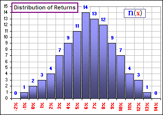
Figure 1
If you add up all the blue numbers you’ll get 100, but many are the same (or, at least they lie in the same small intervals … near 5%, 6%, 7%, etc.). It’d mean that the SUM of logarithms (as indicated by (2), above) has terms like:
… + 11*log(1+0.05) + 14*log(1+0.06) + 13*log(1+0.07) + …
which is a SUM of terms which look like: n(x)*log(1+x) where n(x) is the number of terms which have the same x-value. For simplicity, we’ll write the SUM as S n(x)*log(1+x). Is that okay, for an example?
Yes, please continue.
Okay, in general we have, continuing from (2) above:
(3) log(G) = S n(x)*log(1+x).
Now, if the various values of x are small(remembering that a 9% return would have x = 0.09), then
(4) log(1+x) = x – x2/2 + x3/3 – x4/4 + x5/5 –
You’re assuming natural logarithms, to the base e?
Of course. Is there any other kind? Notice how well the terms up to x4/4 approximate log(1+x)
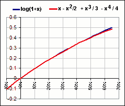
Figure 2
Now we can rewrite equation (3) like so:
(5) log(G) = Sxn(x)-(1/2)S x2 n(x)+(1/3)S x3 n(x)-(1/4)S x4 n(x)+(1/5)S x5 n(x) – …
If the total number of returns is N, then the SUM of all the n(x) is N and, in particular, n(x)/N is the fraction of terms associated with the same x-value. We’ll call this fraction f(x), so
(6) f(x) = n(x)/N.
Now we divide equation (5) by N and get:
(7) log(G)/N = log(G1/N)
= S x f(x)-(1/2)S x2 f(x)+(1/3)S
x3 f(x)-(1/4)S x4 f(x)+(1/5)S x5 f(x)- …
so we have:
(8) G1/N = EXP{S x f(x)-(1/2)S x2 f(x)+(1/3)S x3 f(x)-(1/4)S x4 f(x)+ … }
Figure 2A shows a picture of the relative size of the terms.
zzzZZZ
Wait! We’re almost there! If the x-values are annual returns:
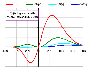
Figure 2A
G1/N is the Annualized Return
S x f(x), the first moment, is the MEAN of the returns: M
S x2 f(x), the second moment, will give the VARIANCE
… or the square of the Standard Deviation: S
S x3 f(x), the third moment, will give the SKEW
S x4 f(x), the fourth moment, will give the KURTOSIS
Will give? What does that mean? Will give … what …?
One usually doesn’t use the raw moments, except for the MEAN, but normalizes or standardizes them. For example, here’s a couple of distributions which look identical except that the MEAN has changed by +30% (or 0.30) … and that has shifted the chart due East by the same amount:
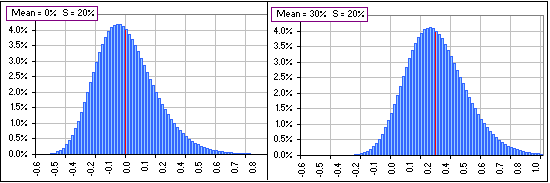
Figure 3
In order to ignore this shift when the MEAN changes (since we’re interested in the “shape” of the distribution, not where it’s located), we can replace x by (x – M) so we’re measuring the deviation of the returns from their MEAN. Then, when we change the MEAN (by, for example, adding a constant amount to each return), the chart will continue to look just like the left chart above (where the MEAN is 0).
And if we change the Standard Deviation? What then?
I was just getting to that. Here’s what’d happen when we change the value of S:
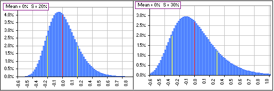
Figure 4
What’re the yellow stripes?
They’re one Standard Deviation, S, above and below the MEAN. You’ll notice that by dividing by N, as in f(x) = n(x)/N, we’ve changed the number of returns lying near an x-value to the fraction of returns lying near an x-value. That makes our analysis independent of the number of returns. In fact, the vertical scale in our distribution charts always run from 0 to 1 (or 0% to 100%).
N could be 100 or 1000 or 10,000 or …
Yes, yes, but now we should do likewise for the horizontal scale. We need some standardized horizontal measure. After all, people use this stuff when the horizontal numbers aren’t annual returns but maybe degrees Fahrenheit or kilograms or maybe miles or hours or …
How about choosing “1” as the horizontal standard?
Well, that’s close to what we’ll do. When x = M + S then …
So x is at a yellow stripe?
Yes. Then we’ll call that “1” unit from the MEAN. To do this we not only replace x by (x-M) … to shift the chart so the “new” mean is zero … but we’ll also replace x by y = (x-M)/S so that …
So that when x=M+S then it’s “1” unit from the MEAN.
Well, y = 1, where y = (x-M)/S is our new horizontal scale. It has the advantage (over x) in that it’s dimensionless. It’ll have the same value whether x is measured in centimetres, miles or light-years.
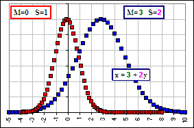
Figure 4A
Indeed, when generating a distribution from scratch, one often defines a standardized distribution for the y’s, then use x = M + y*S to calculate x. For example, if we want to generate a Normal distribution with MEAN = M and Standard Deviation = S, then we get a bunch of y’s from a standard Normal distribution (with M=0, S = 1), then get the x’s via x = M + y*S and the x’s will have MEAN = M and SD = S. In MS Excel, the function NORMSINV(RAND()) returns a standard Normal distribution (with Mean = 0, Standard Deviation = 1) whereas M+S*NORMSINV(RAND()) returns Normally distributed numbers with Mean=M and SD = S.
For example, suppose we plot the fraction of numbers (x’s or y’s) with a particular value, we’d get two curves (as in Figure 4A where the y’s are a standard Normal distribution and the x’s have M = 3 and S = 2). The right curve is the left curve shifted right by 3 and the horizontal dimension stretched by a factor 2. The vertical dimension, which measures the fraction of x’s or y’s which have a particular value, doesn’t change.
I thought the area under the curve must be “1”, no?
Well, there are the same number of x’s as y’s (for example: 100 of each) so the fraction (or percentage) having a particular value is the same … and that’s the vertical value. On the other hand, one usually sees the vertical dimension as the probability density and …
Yeah! That’s what I’m talking about! The density!
Okay. If we have jillions (or an infinity) of numbers then we might want to consider the fraction (or percentage) lying within some interval along the horizontal axis (as opposed to the fraction having one of N = 100 values).
Like: “How many lie between x = 1.0 and x = 1.2”, eh?
Well, not “How many?”. The answer to that question might be “Infinity.
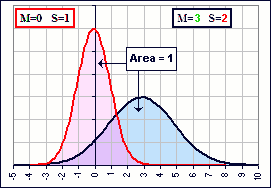
Figure 4B
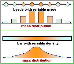
Figure 4C
More like “What percentage?”. In that case the area under the curve must be “1” so, when we stretch the horizontal distance by S, we must shrink the vertical dimension by S as we have in Figure 4B which shows the probability density. It’s like, if you have a rectangle and you increase the width by some factor, then you must decrease the height by the same factor in order to retain the same area.
The use of density is appropriate when you’ve got lots of numbers. For example, if we have a bunch of beads on a string we might plot the mass of the beads, as we move along the string. If, instead, we have a bar of metal with variable density (like: aluminum at the ends changing continuously to gold at the centre), then we’d be better off considering the change of density (meaning the mass per unit length) as we move along the bar.
I’ll take the centre!
Are you paying attention? For a Normal distribution (Mean = M and SD = S), the density is given by:
A: f(x) = {1/(sqrt(2p) S)} e-{(x-M)/S}2/2
After standardization (Mean = 0 and SD = 1) we’d have:
B: f(y) = 1/(sqrt(2p)) e-y2/2
Notice the division by S, in (A). (This f is not to be confused with the earlier f which ain’t a density !)
That is really confusing, I mean …
The earlier f is okay for measuring the mass distribution for beads on a string. The f(x) and f(y) in A and B, above, are appropriate for continuous mass distributions.
Okay, why should the Standard Deviation be used as a horizontal distance?
Why not a vertical … ?
Excellent point. I forgot to mention that S, the Standard Deviation, is a measure of how far the x-values are from their MEAN. In fact, S2 is the average squared distance from the MEAN:
(9) (1/N) {(x1-M)2 + (x2-M)2 + … + (xN-M)2} = S2
or, in terms of our new standardized numbers:
(10)(1/N) {(x1-M)2/S2 + (x2-M)2/S2 + … + (xN-M)2/S2} = (1/N){y12 + y22 + … +yN2}
= 1
Notice that (according to equation 10), points with coordinates (y1, y2, y3, … yN), in N-dimensional space, lie on a hyper-sphere of radius SQRT(N). The greater the number of points, the greater the dimension N, the farther from the origin. That observation is connected to Einstein’s analysis of a random walk or Brownian Motion and how far you’d expect to be from the origin (where you started) after N random steps and …
Let’s not get off track, okay?
What’s the Standard Deviation of these new numbers, y1 and y2 and so on?
One.
One what?
Equation (10) says it all. The MEAN of these new y’s is the number “0” (because we’ve subtracted M from all the x’s) … and the Variance (hence the Standard Deviation) of the y’s is the number “1” (because we’ve divided by S). Note, too, that if x were measured in kilometres (instead of return percentages) then M and S would be in kilometres and they’d all change if we changed the units to miles. However, y = (x-M)/S would have the same value in kilometres as in miles. Nice, eh?
And if x were in degrees Fahrenheit then …
Then we could change to Celsius and, although the x-values would change, the y-values wouldn’t. If we change to y-variables in Figure 1, where y = (x-0.064)/0.029, and we change the vertical coordinate to percentages (so 14-out-of-100 becomes 14%), we’d get Figure 5:
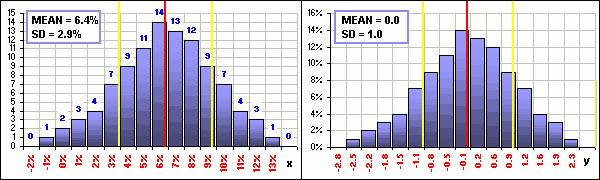
Figure 5
The right chart is standardized. If we add some number (like 15%) to every x, the right chart wouldn’t change. If we multiply every x by some number (like 12), the right chart wouldn’t change. If x was the high temperature each Christmas for the past 100 years, measured in degrees Celsius, and we changed to degrees Fahrenheit, the right …
The right chart wouldn’t change. Yeah, right, okay … I get it!
Good for you.
Okay, so what’s KURTOSIS?
M = (1/N) {x1 + x1 + … +xN} is the MEAN of the x’s.
S = SquareRoot[1/N){(x1-M)2 +(x2-M)2 + … + (xN-M)2}] is the Standard Deviation of the x’s.
then SKEW = (1/N)S yk3 = (1/N)[((x1-M)/S)3 +((x2-M)/S)3 + … + ((xN-M)/S)3]
and KURTOSIS = (1/N)S yk4 = (1/N) [ ((x1-M)/S)4 + ((x2-M)/S)4 + … + ((xN-M)/S)4]
Notice that, after changing from the x’s to the y’s, we’d have a set of y’s with MEAN = 0 (that’s the first moment of the y’s) and Standard Deviation = 1 (that’s the second moment of the y’s) and the third and fourth moments of the y’s give the SKEW and KURTOSIS for the y’s … and for the x’s !
Look carefully at the SKEW. If the x-distribution is symmetrical about the MEAN, then the distribution of x-values above the MEAN is the same as below. This gives rise to positive and negative y-values, hence positive and negative values for y3, and they cancel out, making SKEW = 0. That’s the case for the Normal Distribution. On the other hand, if the distribution is more heavily weighted below the MEAN, the negative values for y3 predominate and that’ll give a negative SKEW. More above and you get a positive SKEW.
Look also at the KURTOSIS definition. It involves the 4th power of the deviation from the MEAN (so they’re always positive) and, if there are more and more x-values far from the MEAN, they contribute significantly to the sum of the y4-values … and the KURTOSIS increases. KURTOSIS is then a measure of how big the “tails” are. Remember Figure 1? Well, the MEAN and Standard Deviation for the x’s are: M = 6.4% and S = 2.9% and if we calculate the SKEW and KURTOSIS, then make some changes in the x-values far from the MEAN … voila!
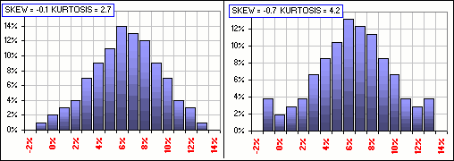
Figure 6
Your charts are all inventions. Haven’t you got a real, live …?
On the right are General Electric stock prices, involving about a thousand daily returns.
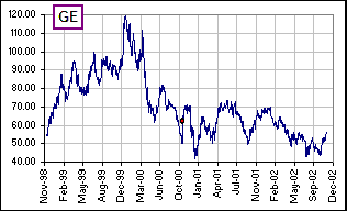
Figure 7A
Below, the distribution of these daily returns for GE, along with a Normal and Lognormal distribution with the same MEAN and Standard Deviation – for comparison purposes. (Nobuddy is suggesting that the GE distribution is one or t’other, but it’s interesting to note that there’s little to choose between normal and lognormal distributions, though neither is a very good representation for the GE distribution):
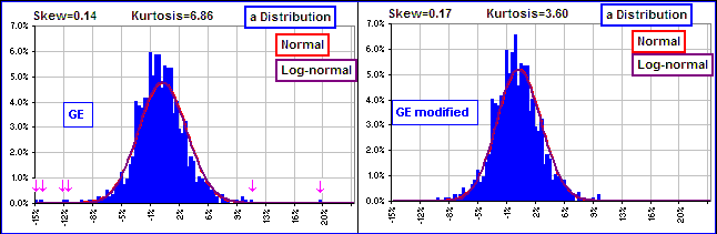
Figure 7B
The left chart gives the actual distribution: KURTOSIS = 6.86. See the outliers- those returns way out on the tails of the distribution, at -15% and -12% and even one at about +20%?
20% for a daily return? You’re kidding, right?
It was October 19, 2000. GE had closed at $51.75 on the 18th and at $61.88 on the 19th. That’s almost a 20% jump (shown as a red dot in Figure 7A). This, together with a few more large changes, make for a big KURTOSIS. However, if we replace a half dozen of these way-out daily returns by 0%, we get the right chart. The outliers are gone, there are more returns at 0% and a we’ve got a smaller KURTOSIS.
At 3.60 it still seems big to me.
Actually, for the Normal Distribution (which is perfectly symmetrical about the MEAN), KURTOSIS = 3.0 and, for this reason, KURTOSIS is sometimes defined to be:
(11) KURTOSIS = (1/N)S yk4 – 3 = (1/N)S {(xk-M)/S}4 – 3
which, by subtracting “3”, gives the deviation from the value for the Normal Distribution. With this definition, the Normal Distribution has a KURTOSIS = 0.
Which one do you use?
I don’t use either. I just regurgitate what others say … just in case you run across one or the other in your travels.
Why the two definitions?
Why are you asking me? But I can tell you, there are other definitions too. Want to see them?
Definitely not!
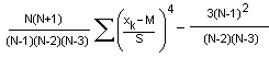
Okay, here’s another. The MS Excel definition:
Gee, thanks. I needed that.
However, for large values of N, it looks like 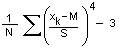 which you’ll recognize from (11) above, right?
Wrong! And by the way, what about S y5 … that fifth moment? What’s its name?
I have no idea.
What? All this and you don’t have a name for it? You should really look up the name before you start writing tutorials. I can’t believe you’d go through all that stuff and not have a name. People like names. They’re important! Haven’t you noticed that? You see a strange bird and everybody says “What is it?” and they’re not satisfied until you say, “a South American Twiddlewot” then they’re all happy, they have a name and they’re satisfied and they don’t need any more information about the Twiddlewot, just a name because …